<?xml version="1.0" encoding="utf-8"?><feed xmlns="http://www.w3.org/2005/Atom" ><generator uri="https://jekyllrb.com/" version="3.10.0">Jekyll</generator><link href="https://deaneyang.github.io//blog/feed.xml" rel="self" type="application/atom+xml" /><link href="https://deaneyang.github.io//blog/" rel="alternate" type="text/html" /><updated>2026-05-14T02:18:08+00:00</updated><id>https://deaneyang.github.io//blog/feed.xml</id><title type="html">A Cluttered Mind</title><subtitle>Math, anecdotes, recipes</subtitle><entry><title type="html">Characterization of Tensor Fields</title><link href="https://deaneyang.github.io//blog/blog/math/differential-geometry/tensors/differential-forms/2026/05/01/TensorFields.html" rel="alternate" type="text/html" title="Characterization of Tensor Fields" /><published>2026-05-01T00:00:00+00:00</published><updated>2026-05-01T00:00:00+00:00</updated><id>https://deaneyang.github.io//blog/blog/math/differential-geometry/tensors/differential-forms/2026/05/01/TensorFields</id><content type="html" xml:base="https://deaneyang.github.io//blog/blog/math/differential-geometry/tensors/differential-forms/2026/05/01/TensorFields.html"><![CDATA[<p>$\newcommand\R{\mathbb{R}}\newcommand\C{\mathbb{C}}\newcommand\Z{\mathbb{Z}}\newcommand\Q{\mathbb{Q}}$</p>

<h4 id="characterization-of-1-forms">Characterization of $1$-forms</h4>

<p>
Let $M$ be a smooth manifold, $T_*M$ be its tangent bundle, and $T^*M$ be its cotangent bundle. For each $p \in M$, $v\in T_pM$ and $\ell\in T_p^*M$, let both $\langle \ell,v\rangle$, and $\langle v,\ell\rangle$ denote the value of $\ell$ with input $v$.
</p>

<p>
Denote
\begin{align*}
  C^\infty(M) &amp;= \text{ space of smooth functions on }M\\
  \Gamma(T_*M) &amp;=\text{ space of smooth vector fields}\\
  \Gamma(T^*M) &amp;=\text{ space of smooth $1$-forms}
\end{align*}
Observe that these satisfy the following property: If $v_1,v_2$ are vector fields, $\theta_1,\theta_2$ are $1$-forms, and $f_1,f_2$ are smooth functions, then
\begin{align*}
  f_1v_1 + f_2v_2 &amp;\in \Gamma(T_*M)\\
  f_1\theta_1 + f_2\theta_2 &amp;\in \Gamma(T^*M).
\end{align*}
</p>

<p>
<b>Definition.</b> A map
$$ A: \Gamma(T_*M) \rightarrow C^\infty(M) $$
is <b>${\mathbf C^\infty(M)}$-linear</b> if for any $v_1,v_2\in\Gamma(T_*M)$ and $f_1,f_2\in C^\infty(M)$,
$$ A(f_1v_1+f_2v_2) = f_1A(v_1)+f_2(v_2). $$
This is a globally defined property of $A$.
</p>

<p>
The tensor characterization lemma states that for each $p\in M$, the value of $A(v)(p)$ depends only on the value of $v$ at $p$ and not on the value of $v$ elsewhere. More precisely, it states the following:
</p>

<p>
<b>Lemma.</b>
<em>A map (i.e., operator)
  \begin{align*}
  A: \Gamma(T_*M) \rightarrow C^\infty(M)
\end{align*}
is $C^\infty(M)$-linear if and only if there exists a $1$-form $\alpha\in\Gamma(T^*M)$ such that for each $p\in M$ and $v\in\Gamma(T_*M)$,
\[
  A(v)(p) = \langle \alpha(p),v(p)\rangle.
\]
</em>
</p>

<p><b>Proof of Lemma.</b>
Given a smooth $1$-form $\alpha$, the map $A$ given by
\begin{align*}
  A(v)(p) = \langle\alpha(p),v(p)\rangle
\end{align*}
is clearly $C^\infty(M)$-linear.
</p>

<p>
The converse follows by writing everything with respect to a frame of vector fields and its dual coframe.
</p>

<p>
Let $p\in M$. Let $s_1,\dots,s_n$ be smooth vector fields on $M$ such that $(s_1(p),\dots,s_n(p))$ is a basis of $T_pM$, and let $(\sigma^1_p,\dots,\sigma^n_p)$ be the dual basis.
</p>
<p>
Given a $C^\infty(M)$-linear map $A: \Gamma(T_*M) \rightarrow C^\infty(M)$, let
\begin{align*}
a_k &amp;= A(s_k),\ 1 \le k \le n\\
\alpha_p &amp;= a_1(p)\sigma^1_p+\cdots+a_n(p)\sigma_p.
\end{align*}
Given a vector field $v$ on $M$, let $f^1,\dots,f^n\in\C^\infty(M)$ satisfy
$$ v(p) = f^1(p)s_1(p)+\cdots+f^n(p)s_n(p). $$
Observe that
\begin{align*}
\langle\alpha_p,v(p)\rangle &amp;= \langle a_1(p)\sigma^1_p+\cdots+a_n(p)\sigma^n_p,f^1(p)s_1(p)+\cdots+f^n(p)s_n(p)\rangle\\
&amp;= a_1(p)f^1(p)+\cdots+a_n(p)f^n(p).
\end{align*}
It follows that
\begin{align*}
A(v)(p) &amp;= A(f^1s_1+\cdots+f^ns_n)(p)\\
&amp;= (f^1A(s_1)+\cdots+f^nA(s_n))(p)\\
&amp;= f^1(p)a_1(p)+\cdots+f^n(p)a_n(p)\\
&amp;= \langle\alpha_p,v(p)\rangle.
\end{align*}
This implies that for each $p \in M$, there exists a unique $\alpha_p\in T_p^*M$ such that for any vector field $v$,
\begin{align*}
A(v)(p) &amp;= \langle\alpha_p,v(p)\rangle.
\end{align*}
Let $\alpha$ be the $1$-form given by
$$ \alpha(p) = \alpha_p,\ p\in M. $$
That $\alpha$ is smooth follows from the fact that $A(v)(p)$ is a smooth funcction of $p$.
</p>

<p>
<b>Q.E.D.</b>
</p>

<h4 id="characterization-of-k-tensor-fields">Characterization of $k$-tensor fields</h4>

<p>
Recall that if $k\ge 1$, then a <b>$\mathbf{k}$-tensor $\Theta$ on a vector space $V$</b> is a multilinear function
\begin{align*}
  \Theta: V\times\cdots\times V &amp;\rightarrow \R
\end{align*}
with $k$ inputs. The space of all $k$-tensors is a vector space, which we will denote by $\otimes^k V^*$. Observe that $\otimes^1V^* = V^*$. As a convention, we also let $\otimes^0V^* = \R$.
</p>

<p>
At each $p \in M$, a <b>$\mathbf{k}$-tensor</b> is a $k$-tensor over the vector space $T_pM$, i.e., an element of $\otimes^kT_p^*M$. Let
\begin{align*}
  \otimes^kT^*M = \coprod_{p\in M} \otimes^kT_p^*M.
\end{align*}
A local trivialization of $T_*M$ can be used to define a local trivialization of $\otimes^kT^*M$ and therefore $\otimes^kT^*M$ is a vector bundle, which we call the $k$-tensor bundle. See below for a proof.
</p>

<p>
A <b>$\mathbf{k}$-tensor field</b> is a smooth section of $\otimes^kT^*M$, i.e., a map
\begin{align*}
  \theta: M \rightarrow \otimes^kT^*M
\end{align*}
such that for each $p \in M$,
\begin{align*} \theta(p)\in\otimes^kT^*_pM. \end{align*}
The space of $k$-tensor fields satisfies the following property: If $\Theta_1,\Theta_2\in\Gamma(\otimes^kT^*M)$ and $f_1,f_2\in C^\infty(M)$, then
\begin{align*} f_1\Theta_1+f_2\Theta_2 \in \Gamma(\otimes^kT^*M). \end{align*}
</p>

<p>
 A map
  \begin{align*}
  \Theta: \Gamma(T_*M)\times\cdots\Gamma(T_*M) \rightarrow C^\infty(M)
\end{align*}
with $k$ inputs
is <b>$\mathbf{C^\infty(M)}$-linear</b> if for any vector fields $v_1,\dots,v_k$ and functions $f^1,\dots,f^k$,
\begin{align*}
\Theta(f^1v_1+\cdots+f^nv_n) = f^1\Theta(v_1)+\cdots+f^k\Theta(v_k).
\end{align*}
</p>

<p>
<b>Lemma.</b> A map
  \begin{align*}
  \Theta: \Gamma(T_*M)\times\cdots\Gamma(T_*M) \rightarrow C^\infty(M)
\end{align*}
is $C^\infty(M)$-linear if and only if there exists a $k$-form $\theta$ such that for each $p\in M$ and vector fields $v_1,\dots,v_k$,
\[
  \Theta(v_1,\dots,v_k)(p) = \theta(p)(v_1(p),\dots,v_k(p)).
\]
</p>

<p>
<b>Proof.</b> It is straightforward to adapt the proof for $1$-forms to $k$-forms. <b>Q.E.D</b>
</p>

<h3 id="appendix">Appendix</h3>

<h4 id="otimesktm-is-a-vector-bundle">$\otimes^kT^*M$ is a vector bundle</h4>

<p>Coming soon</p>]]></content><author><name></name></author><category term="blog" /><category term="math" /><category term="differential-geometry" /><category term="tensors" /><category term="differential-forms" /><summary type="html"><![CDATA[$\newcommand\R{\mathbb{R}}\newcommand\C{\mathbb{C}}\newcommand\Z{\mathbb{Z}}\newcommand\Q{\mathbb{Q}}$]]></summary></entry><entry><title type="html">Exponential functions and Euler’s formula</title><link href="https://deaneyang.github.io//blog/blog/math/exponential-function/euler-formula/2025/05/29/ExponentialFunctions.html" rel="alternate" type="text/html" title="Exponential functions and Euler’s formula" /><published>2025-05-29T00:00:00+00:00</published><updated>2025-05-29T00:00:00+00:00</updated><id>https://deaneyang.github.io//blog/blog/math/exponential-function/euler-formula/2025/05/29/ExponentialFunctions</id><content type="html" xml:base="https://deaneyang.github.io//blog/blog/math/exponential-function/euler-formula/2025/05/29/ExponentialFunctions.html"><![CDATA[<p>$\newcommand\R{\mathbb{R}}\newcommand\C{\mathbb{C}}\newcommand\Z{\mathbb{Z}}\newcommand\Q{\mathbb{Q}}$</p>

<p>
This post was driven by a desire to explain  and prove Euler's formula,
\begin{equation}\label{euler}
e^{i\theta} = \cos\theta + i\sin \theta,
\end{equation}
in a more conceptual way than the standard explanation using power series. Power series are still used as the key technical tool for proving the existence and uniqueness of exponential functions.
</p>

<p><b>Acknowledgements.</b> <i>This was provoked by a <a href="https://www.quantamagazine.org/how-infinite-series-reveal-the-unity-of-mathematics-20220124/">Quanta Magazine article by Steven Strogatz on how to prove Euler's formula using power series.</a> The discussion below was inspired by Michael Hutchings' observation that Euler's formula can be proved by solving an ordinary differential equation.</i> I'd also like to thank Dan Lee, Keith Conrad, and my other Facebook friends for their comments and corrections.</p>

<h3 id="introduction">Introduction</h3>

<p>
At first, even the meaning of the left side of Euler's formula \eqref{euler} is unclear. The standard approach is to use power series to define $e^{i\theta}$ and prove Euler's formula. The argument is outlined below. It is simple and elegant. I have, however, always found it unsatisfying, since the power series alone provides little intuition into what's going on.
</p>

<p>
Here, I provide an alternative approach that I find that is easier to understand intuitively. Moreover, it accomplishes much more. Using only calculus, it provides rigorous definitions of not only the exponential, sine, and cosine functions, but also the constants $\pi$ and $e$. From these definitions, it is straightforward to prove the fundamental properties of these functions, including Euler's formula.
</p>

<p>
It is worth noting that the standard way to define the sine and cosine functions requires the concept of an angle, in degrees or radians, but no rigorous definition is provided This in fact is not easy to do and rarely discussed at all in calculus textbooks. Here, we start with the definition of $e^{i\theta}$ and use it to define rigorously what the sine and cosine functions, as well as angles, are.
</p>

<p>
The exposition here does not require the use of power series. Power series are needed only for proving rigorously the existence of exponential functions. The details of this have been relegated to the Appendix.
</p>

<h3 id="power-series-proof-of-eulers-formula">Power series proof of Euler’s formula</h3>

<p>
Here is a brief outline of how to prove Euler's formula using power series. The starting point are the power series
\begin{align}
  e^{x} &amp;= \sum_{k=0}^\infty \frac{x^k}{k!} = 1 + x + \frac{x^2}{2!} +\cdots \label{taylor}\\
  \sin x &amp;= \sum_{k=0}^\infty (-1)^k\frac{x^{2k+1}}{(2k+1)!}
  = x - \frac{x^3}{3!} + \frac{x^5}{5!} + \cdots \notag\\
  \cos x &amp;= \sum_{k=0}^\infty (-1)^k\frac{x^{2k}}{(2k)!}
  = 1 - \frac{x^2}{2!} + \frac{x^4}{4!} + \cdots. \notag
\end{align}
It follows by the ratio test that these series converge for every $x \in \R$.
The key observation is that these power series also converge if $x$ is complex, extending the domains of these functions from $\R$ to $\C$. 
 Euler's formula now follows by setting $x = i\theta$ in \eqref{taylor} and splitting the series into its real and imaginary parts,
\begin{align*}
e^{i\theta} &amp;= \sum_{k=0} \frac{(i\theta)^k}{k!}\\
            &amp;= \sum_{k=0} (-1)^k \frac{\theta^{2k}}{(2k)!}
            + i\sum_{k=0} (-1)^k \frac{\theta^{2k+1}}{(2k+1)!}\\
            &amp;= \cos\theta + i\sin\theta.
\end{align*}  
This is simple and elegant, but the proof provides little intuition to what is going on. Euler's formula appears magically.
</p>

<p>
Below is an alternative approach that I think elucidates how the exponential function of both real and imaginary numbers arise and why exponential of an imaginary number has a geometric interpretation. The explanation below requires only basic calculus. No knowledge of differential equations is needed. The appendix provides a rigorous discussion showing how to use power series to solve a simple ordinary differential equation. The uniqueness of the solution follows from basic properties of the integral.
</p>

<h3 id="exponential-function-of-a-real-number">Exponential function of a real number</h3>

<p>We start by recalling what a real exponential function is.</p>

<h4 id="linear-function">Linear function</h4>

<p>
We start by with the definition of a linear function. A function $f: \R \rightarrow \R$ is <b>linear</b> if the change in output depends only on the change in input and not on the input itself. More precisely, for any change in input, $\Delta \ne 0$, there exists $c(\Delta) \in \R$ such that
$$
f(x+\Delta) - f(x) = c(\Delta),\ \forall x \in \R
$$
Observe that $c(0) = 0$. Therefore, if $f$ is assumed to be differentiable, then
\begin{align*}
f'(x) &amp;= \lim_{\Delta\rightarrow 0} \frac{f(x+\Delta)-f(x)}{\Delta}\\
&amp;= \lim_{\Delta\rightarrow 0} \frac{c(\Delta)-c(0)}{\Delta}\\
&amp;= c'(0),
\end{align*}
which is a constant. If we set $m = c'(0)$ and $b = f(0)$, this implies that if $f$ is linear, then
$$ f(x) = mx + b. $$
The converse also holds.
</p>

<h4 id="exponential-functions">Exponential functions</h4>

<p>
An exponential function has a similar definition except that change in output is replaced by relative change in input. In other words, a function $E: \R \rightarrow \R$ is <b>exponential</b> if the <b>percentage or relative change</b> of $E$ depends only on the change in input and not on the input itself. More precisely, for any $\Delta \in \R$, there exists $C(\Delta)$ such that
\begin{equation}\label{relative-change}
\frac{E(x+\Delta)-E(x)}{E(x)} = C(\Delta).
\end{equation}
Observe that $C(0) = 0$.
From this, it follows that, if $E$ is differentiable, then
\begin{align*}
\frac{E'(x)}{E(x)} &amp;= \lim_{\Delta\rightarrow 0}\frac{E(x+\Delta)-E(x)}{E(x)\Delta}\\
      &amp;= \lim_{\Delta\rightarrow 0}\frac{C(\Delta)-C(0)}{\Delta}\\
      &amp;= C'(0)
\end{align*}
This implies that $C(\Delta)$, as a function of $\Delta$, is differentiable at $\Delta = 0$, and
\begin{equation}\label{exponential}
E'(x) = \kappa E(x),
\end{equation}
where $\kappa = C'(0)$ is a constant.
</p>

<p>
Any function $E$ on a nonempty connected interval $I$ that satisfies \eqref{exponential} for some constant $\kappa$ is called an <b>exponential function</b>. Observe that if $\kappa = 0$, then $E$ is a constant function.
</p>

<h4 id="existence-of-exponential-functions">Existence of exponential functions</h4>

<p>The following is proved in the appendix:</p>
<div class="theorem">
Given any $\kappa, e_0 \in \R$, there exists a differentiable function $E: \R \rightarrow \R$ satisfying
\begin{equation}\label{ode}
E' = \kappa E\text{ and }E(0) = e_0.
\end{equation}
</div>

<h4 id="properties-of-exponential-functions">Properties of exponential functions</h4>

<p><b>Product of exponential functions is exponential:</b>
Let $E_1$ and $E_2$ be exponential functions that satisfy
$$ E_1' = \kappa_1E_1 \text{ and } E_2' = \kappa_2E_2. $$
If $E_3 = E_1E_2$, then
\begin{align*}
E_3' &amp;= E_1'E_2 + E_1E_2'\\
&amp;= (\kappa_1+\kappa_2)E_1E_2\\
&amp;= \kappa_3 E_3,
\end{align*}
where $\kappa_3 = \kappa_1+\kappa_2$.
</p>

<p>
A special case is when
$$ E_1'=\kappa E_1\text{ and }E_2=-\kappa E_2$$ on a nonempty connected open interval $I$. In that case, the product $E_1E_2$ is a constant function. This leads to the following:
</p>

<p>
<b>An exponential function is either always or never zero:</b>
<i>If $E' = \kappa E$ on a nonempty connected open interval $I$, then either $E=0$ on $I$ or $E$ is never zero on $I$.</i></p>

<p><b>Proof:</b> Suppose there exists $t_0 \in I$ such that $E(t_0) = e_0 \ne 0$. Let $E_2$ be the exponential function given by
$$E_2' = -\kappa E_2\text{ and }E_2(t_0) = 1. $$
This implies that for any $t \in I$,
$$ E(t)E_2(t) = e_0. $$
Therefore, $E(t) \ne 0$ for each $t \in I$.
</p>

<p>
The properties above imply the uniqueness of a solution to \eqref{ode}. See the Appendix for a proof.
</p>

<h4 id="standard-exponential-functions">Standard exponential functions</h4>

<p>
Given $\kappa \in \R$, let $e_\kappa: \R \rightarrow \R$ denote the unique function such that
\begin{equation}\label{ode1}
e_\kappa' = \kappa e_\kappa\text{ and }e_\kappa(0) = 1
\end{equation}
</p>

<p>
Observe that if $E(x) = e_1(\kappa x)$, then
$$
E'(x)=\kappa e_1'(\kappa x) = \kappa e_1(\kappa x) = \kappa E\text{ and }E(0)=1.
$$
By the uniqueness of a solution to \eqref{ode1}, it follows that $E = e_\kappa$ and therefore
$$
e_\kappa(x) = e_1(\kappa x),\ \forall x \in \R.
$$
</p>

<p>An important property of a standard exponential function is the following:</p>

<p>
\begin{equation}\label{translation}
e_\kappa(s+t) = e_\kappa(s)e_\kappa(t)
\end{equation}
This follows from the fact that if $s$ is held fixed, then the two sides of the equation are solutions to \eqref{ode} and therefore have to be equal.
</p>

<h4 id="eulers-constant-e">Euler’s constant $e$</h4>

<p>We define Euler’s constant to be
\(e = e_1(1).\)</p>

<p>
It follows by \eqref{translation} that for any nonnegative integer $k$,
$$ e_1(k+1) = e_1(k). $$
By induction and that $e_1(0)=0$, it follows that
$$ e_1(k) = e^k. $$
Also, since
$$ 1 = e_1(0) = e_1(k+(-k)) = e_1(k)e_1(-k), $$
it follows that for any positive integer $k$,
$$ e_1(-k) = e^{-k}. $$
Therefore, for any integer $k$,
$$ e_1(k) = e^k. $$
</p>

<p>
For any rational number $\frac{n}{d}$, where $n$ is an integer and $d$ is a positive integer,
\begin{align*}
e^n &amp;= e_1(n)\\  &amp;= e_1\left(\frac{n}{d}+\cdots+\frac{n}{d}\right)\\
&amp;= \left(e_1\left(\frac{n}{d}\right)\right)^d
\end{align*}
It follows that
\begin{align*}
e_1\left(\frac{n}{d}\right) &amp;= (e^n)^{\frac{1}{d}} = e^{\frac{n}{d}}.
\end{align*}
In short, for any rational $r$
$$
e_1(r) = e^r.
$$
</p>

<p>
These properties justify the following definition: For any $x \in \R$, we denote the standard exponential function by
$$
e^x = e_1(x).
$$
Note that if $x$ is irrational, this is the <b>definition</b> of $e^x$.
This function satisfies the following properties:
\begin{align*}
e^x &amp;&gt; 0,\ \forall x \in \R\\
e^0 &amp;= 1\\
e^{x+y} &amp;= e^xe^y,\ \forall x,y \in \R.
\end{align*}
</p>

<p>
Moreover, any exponential function $E: \R \rightarrow \R$ can be written as
$$
E(t) = e_0e^{\kappa t},
$$
where $e_0 = E(0)$ and $\kappa = E'/E$ are constants.
</p>

<h3 id="exponential-of-an-imaginary-number">Exponential of an imaginary number</h3>

<p>
Now suppose you want to extend the definition of $e^t$ to $t \in \C$. Let us focus first on the case $t = i$. One could try to define
$$
e^i = e_1(i).
$$
But this is problematic, because it would mean trying to solve \eqref{ode} with respect to an independent variable $t$ that is complex instead of real. A better approach is to use \eqref{ode} as a template and define
$$
e^i = e_i(1),
$$
where $e_i$ satisfies the equation
\begin{equation} e_i' = ie_i\text{ and }e_i(0) = 1. \label{ode2} \end{equation}
By theorem in the appendix, there is a unique solution $e_i: \R \rightarrow \C$ to \eqref{ode2}. Moreover, for any $t_1, t_2 \in \R$,
$$ e_i(t_1 + t_2) = e_i(t_1)e_i(t_2), $$
which justifies writing, for any $t \in \R$,
$$ e_i(t) = e^{it}. $$
</p>

<h4 id="geometric-properties-of-the-exponential-of-an-imaginary-number">Geometric properties of the exponential of an imaginary number</h4>

<p>
We now want to understand the function $e^{it}$ better. An unexpected twist is that geometry and trigonometry naturally appear in the description of this function.
</p>

<p>
If we write $e_i(t) = x(t) + iy(t)$ and differentiate it, the left side of \eqref{ode2} looks like
\begin{align}
e_i'(t) &amp;= x'(t) + iy'(t).
\end{align}
On the other hand, the right side looks like
\begin{align}
ie_i(t) &amp;= i(x(t)+iy(t))\\
        &amp;= -y(t) + ix(t)
\end{align}
It follows that \eqref{ode2} can be written as
\begin{align}\label{ode7}
x'(t) + iy'(t) &amp;= -y(t) + ix(t).
\end{align}
Since the left side equals the right only if the real parts match and so do the imaginary parts, \eqref{ode7} is equivalent to the equations
\begin{align}\label{ode3}
(x',y') &amp;= (-y,x)\text{ and }(x(0),y(0)) = (1,0).
\end{align}
A solution to this satisfies
\begin{align}\label{perp}
(x',y')\cdot (x,y) = x'x + y'y = -yx + xy = 0.
\end{align}
In other words, $(x(t),y(t))$, $t \in \R$, is a parameterized curve whose velocity vector
$$
v = (x', y')
$$
is always orthogonal to the position vector $(x,y)$.
It is now a straightforward exercise to show that \eqref{perp} implies
\begin{align}
x^2 + y^2 &amp;= 1 \label{unit}\\
(x')^2+(y')^2 &amp;= 1. \label{unit-speed}.
\end{align}
The first equation says the curve always lies on the unit circle centered at the origin. The second says that the speed, which is the norm of the velocity vector, is always equal to $1$.
Equations \eqref{perp}, \eqref{unit}, \eqref{unit-speed} imply that the solution is a unit speed parameterization of the circle.
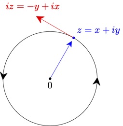
</p>

<p align="center">
  <img src="/blog/assets/images/circle.jpg" style="height:12%;" />
</p>

<p>
Since the parameterization has unit speed, it is intuitively clear that, as $t$ increases, the solution $(x(t),y(t))$ to \eqref{ode3} goes around the entire circle at least once. In particular, there exists $\tau &gt; 0$ such that
$$
e_i(\tau) = e_i(0) = 1.
$$
A rigorous proof of this is provided in the Appendix.
The translation invariance of \eqref{ode2} implies that for any $t \in \R$,
$$
e_i(t + \tau) = e_i(t)e_i(\tau) = e_i(t).
$$
A function with this property is called <b>periodic</b>.
</p>

<h4 id="definition-of-pi">Definition of $\pi$</h4>

<p>
Let $\tau$ be the smallest positive constant such that
$$ e_i(\tau) = 1. $$
The constant $\pi$ is defined to be
$$
\pi = \frac{\tau}{2}.
$$
For each $t \in [0,2\pi]$,
$$ e_i(t) = x(t) + iy(t) $$
is the point reached by traveling at unit speed along the circle staring from $(1,0)$. We can therefore define the <b>length</b> of the arc from $(1,0)$ to $(x(t),y(t))$, where $0 \le t &lt; 2\pi$, to be $t$. In particular, the <b>circumference</b> of the circle, which is defined to be the length of the full circle, is $2\pi$.
</p>

<p>
The <b>angle in radians</b> from $(1,0)$ to the point $(x,y)$ on the unit circle is defined to be the length of the arc from $(1,0)$ to $(x,y)$ and therefore the unique $t \in [0,2\pi)$ such that
$$
e^{it} = x + iy.
$$
</p>

<h4 id="definitions-and-properties-of-trig-functions">Definitions and properties of trig functions</h4>

<p>
We can now define the basic trig functions to be, for any $\theta \in \R$,
\begin{align*}
\cos\theta &amp;= x(\theta)\\
\sin\theta &amp;= y(\theta),
\end{align*}
where
$$
e^{i\theta} = x(\theta) + iy(\theta).
$$
In other words,
$$
e^{i\theta} = \cos\theta + i\sin\theta.
$$
Therefore, the sine and cosine functions are defined using Euler's formula.
</p>

<p>
Straightforward consequences of everything above include
$$ (\sin\theta)^2 + (\cos\theta)^2 = 1, $$
Euler's formula
$$ e^{i\theta} = \cos\theta + i\sin\theta, $$
and the standard differentiation formulas,
\begin{align*}
\frac{d}{d\theta}(\sin\theta) &amp;= \cos\theta\\
\frac{d}{d\theta}(\cos\theta) &amp;= -\sin\theta.
\end{align*}
It is also straightforward to use the symmetries of \eqref{ode2} to derive all of the basic properties of the sine and cosine functions, such as:
\begin{align*}
\sin(n\pi) &amp;= 0\\
\sin\left(\frac{\pi}{2}+2\pi n\right) &amp;= 1\\
\sin\left(\frac{3\pi}{2}+2\pi n\right) &amp;= -1\\
\cos(2n\pi) &amp;= 1\\
\cos((2n+1)\pi) &amp;= -1\\
\cos\left(\frac{\pi}{2}+n\pi\right) &amp;= 0,
\end{align*}
where $n$ is any integer.
Many trigonometric identities also follow easily by raising $e^{i\theta}$ to integer and rational powers.
</p>

<h4 id="exponential-of-a-complex-number">Exponential of a complex number</h4>

<p>
Finally, it is now obvious how to define the exponential of a complex number $z$, namely
$$ e^{z} = e_z(1), $$
where $e_z$ is the unique solution to the ODE
\begin{equation}\label{ode4}
e_z' = ze_z\text{ and }e_z(0) = 1.
\end{equation}
Again, it is straightforward to show that
$$
e^{z_1+z_2} = e^{z_1}e^{z_2}
$$
and, in particular,
$$
e^{x+iy} = e^xe^{iy} = e^x(\cos y + i\sin y)..
$$
</p>

<h3 id="summary">Summary</h3>
<p>
The above shows how to use only calculus to obtain not just definitions but also geometric interpretations of the following:
<ul>
<li>The constants $e$ and $\pi$</li>
<li>The exponential functions $e^t$ and $e^{it}$, for any $t \in \R$</li>
<li>Radians</li>
<li>The trigonometric functions $\sin\theta$ and $\cos\theta$, for any $\theta \in \R$</li>
</ul>
Euler's formula now arises naturally from the definitions of $\sin\theta$ and $\cos\theta$.
</p>

<h3 id="appendix">Appendix</h3>

<h4 id="existence-of-a-solution-to-eqrefode-eqrefode2-or-eqrefode4">Existence of a solution to \eqref{ode}, \eqref{ode2}, or \eqref{ode4}</h4>

<p>Since \eqref{ode} and \eqref{ode2} are special cases of \eqref{ode4}, it suffices to prove the following:</p>

<div class="theorem">
Given $e_0, \kappa \in \C$, there exists a differentiable function $E: \R \rightarrow \C$ satisfying
\begin{equation}\label{ivp}
  E' = \kappa E\text{ and }E(0) = e_0.
\end{equation}
</div>

<div class="proof">
<p> We use power series to prove that a solution to \eqref{ivp} exists.
</p>

<p>Consider the power series
$$
E(t) = \sum_{k=0} c_kt^k.
$$
If $E$ satisfies the equation \eqref{ivp}, then that $c_0 = e_0$ and
$$
\sum_{k=0}^\infty (k+1)c_{k+1}t^k = \sum_{k=0}^\infty \kappa c_kt^k,
$$
which implies that for each $k \ge 0$,
$$
c_{k+1} \frac{\kappa }{k+1}c_k.
$$
By induction, we see that
$$
c_k = e_0\frac{\kappa ^k}{k!},
$$
Therefore, the power series for $E$ is
$$
e_0\sum_{k=0}^\infty \frac{(\kappa t)^k}{k!}.
$$
It is easily checked that by the ratio test for series, the series, for any fixed $t \in \R$, converges absolutely. We can therefore define
$$
E(t) = e_0\sum_{k=0}\frac{(\kappa t)^k}{k!}.
$$
</p>

<p>
It remains to show that $E$ really does satisfy the \eqref{ivp}. First, we derive the power series for $E'$ as follows: 
\begin{align*}
E'(x) &amp;= \lim_{y\rightarrow x} \frac{E(y)-E(x)}{y-x}\\
&amp;= \lim_{y\rightarrow x} \frac{1}{y-x}\left(e_0\sum_{k=0}^\infty \frac{(\kappa y)^k}{k!}
- e_0\sum_{k=0}^\infty \frac{(\kappa x)^k}{k!}\right)\\
&amp;= e_0\lim_{y\rightarrow x} \sum_{k=0}^\infty \frac{1}{k!}\left(\frac{(\kappa y)^k-(\kappa x)^k}{y-x}\right)\\
&amp;= e_0\lim_{y\rightarrow x} \sum_{k=1}^\infty \frac{\kappa^k}{k!}(y^{k-1}+y^{k-2}x + \cdots + yx^{k-2} + x^{k-1})\\
&amp;= e_0\sum_{k=1}^\infty \frac{\kappa^k}{k!}kx^{k-1}\\
&amp;= \kappa e_0\sum_{k=0}^\infty \frac{(\kappa x)^k}{k!}\\
&amp;= \kappa E.
\end{align*}
Since, by the ratio test, all of the series in the calculation above converge absolutely, it is a valid calculation and therefore
$$
E' = \kappa E.
$$
</p>
</div>

<h4 id="uniqueness-of-a-solution-to-eqrefode-eqrefode2-or-eqrefode4">Uniqueness of a solution to \eqref{ode}, \eqref{ode2}, or \eqref{ode4}</h4>

<p>
The proof of existence already implies that \eqref{ode4} has a unique power series solution. However, we want to prove uniqueness assuming only that the solution is differentiable.
</p>

<div class="theorem">
Given $e_0, \kappa \in \C$ and $t_0 &lt; t_1$, if $E_1, E_2: [t_0,t_1] \rightarrow  \C$ are solutions to
\begin{equation}\label{ivp2}
  E' = \kappa E\text{ and }E(t_0) = e_0,
\end{equation}
then $E_1=E_2$.
</div>

<div class="proof">
<p>
We have already shown that if $e_0=0$, then the only solution to \eqref{ivp2} is the zero function. On the other hand, if $e_0 \ne 0$, then $E=E_2-E_1$ satisfies \eqref{ivp2} with $e_0=0$. Therefore, $E$ is the zero function and $E_2=E_1$.
</p>
</div>

<h4 id="a-solution-to-eqrefode3-goes-around-the-whole-circle">A solution to \eqref{ode3} goes around the whole circle</h4>

<p>
<b>Lemma.</b>
Let $C = \{ (x,y) \in \R^2:\ x^2+y^2=1\}$.
Let $(x,y): \R \rightarrow C$ be the unique solution to
\begin{align}\label{ode5}
    (x',y') &amp;= (-y,x)\\
\label{initial}
    (x(0),y(0)) &amp;= (1,0).
\end{align}
</p>

<p>
Then there exists $\tau &gt; 0$ such that
$$
   \left.(x,y)\right|_{[0,\tau)}: [0,\tau) \rightarrow C
$$
is a bijection and $(x(\tau),y(\tau))= (x(0),y(0))$.
</p>

<div class="proof">
  Let $C = C_1 \cup C_2 \cup C_3 \cup C_4$, where
  \begin{align*}
    C_1 = \left\{ (x,y) \in C:\ x \ge \frac{1}{\sqrt{2}} \right\}\\
    C_2 = \left\{ (x,y) \in C:\ y \ge \frac{1}{\sqrt{2}} \right\}\\
    C_3 = \left\{ (x,y) \in C:\ x \le \frac{-1}{\sqrt{2}} \right\}\\
    C_4 = \left\{ (x,y) \in C:\ y \le \frac{-1}{\sqrt{2}} \right\}\\
  \end{align*}

<p align="center">
  <img src="/blog/assets/images/arcs.png" style="height:12%;" />
</p>

  Let
  $$ S = \left\{ T &gt; 0:\ \forall t \in [0,T],\ x(t) \ge \frac{1}{\sqrt{2}}\right\}.$$
  Since $x(0)=1$, $S_1$ is nonempty. Since $y' = x$ and $y(0)=0$, it follows that, for any $T \in S_1$,
  \begin{equation}
    1 \ge y(T) = \int_{t=0}^{t=T} y'(t)\,dt = \int_{t=0}^{t=T} x(t)\,dt \ge \frac{T}{\sqrt{2}}
  \end{equation}
  and therefore
  $$ T \le \sqrt{2}. $$
  Let
  $$ T_+ = \sup S. $$
  If
  $$ y(T_+) &lt; \frac{1}{\sqrt{2}}, $$
  then
  $$ x(T_+) = \sqrt{1-(y(T_+))^2} &gt; \frac{1}{\sqrt{2}}, $$
  which implies that there exists $T &gt; T_+$ such that $T \in S$. This contradicts the definition of $T_+$. Therefore,
  $$ y(T_+) = \frac{1}{\sqrt{2}}. $$

  Let $(x_1,y_1): [-T_+,T_+] \rightarrow C$ be given by
  \begin{align*}
    (x_1(t),y_1(t))
    &amp;=
      \begin{cases}
        (x(-t),-y(-t) &amp;\text{ if }-T_+ \le t \le 0\\
        (x(t),y(t)) &amp;\text{ if }0 \le t \le T_+.
      \end{cases}
  \end{align*}
  It is easy to check that $(x_1,y_1)$ is a solution to \eqref{ode5} and \eqref{initial} on the interval $[-T_+,T_+]$ and, therefore,
  $$ (x_1,y_1) = \left.(x,y)\right|_{[-T_+,T_+]}. $$
  For each $t \in [-T_+,T_+]$,
  \begin{align*}
    y'(t) = x(t) &amp;\ge \frac{1}{\sqrt{2}}
  \end{align*}
  and
  \begin{align*}
    y(-T_+) &amp;= -\frac{1}{\sqrt{2}}\\
    y(T_+) &amp;=\frac{1}{\sqrt{2}}.
  \end{align*}
  It follows that 
  $$ \left.(x,y)\right|_{[-T_+,T_+]}: [-T_+,T_+] \rightarrow C_1 $$
  is a bijection.

  Next, the map $(x_2,y_2): [T_+,3T_+] \rightarrow C$ given by
  $$ (x_2(t),y_2(t) = (-y(t-2T_+),x(t-2T_+)) $$
  satisfies
  \begin{align*}
    y_2(t) &amp;\ge \frac{1}{\sqrt{2}}\\
    x_2'(t) &amp;= -y'(t-2T_+) = -x(t-2T_+) = -y_2(t) &lt; 0\\
    (x_2(T_+),y_2(T_+)) &amp;= (-y(-T_+),x(-T_+)) = \left(\frac{1}{\sqrt{2}},\frac{1}{\sqrt{2}}\right)\\
    (x_2(3T_+),y_2(3T_+)) &amp;= (-y(T_+),x(T_+)) = \left(\frac{-1}{\sqrt{2}},\frac{1}{\sqrt{2}}\right).
  \end{align*}
  It is therefore a bijective map from $[T_+,3T_+]$ to $C_2$.
  It is also a solution to \eqref{ode5} such that
  $$ (x_2(T_+),y_2(T_+)) = (x(T_+),y(T_+)). $$
  Therefore,
  $$ (x_2,y_2) = \left.(x,y)\right|_{[T_+,3T_+]}. $$
  Similar arguments show tht the maps
  \begin{align*}
    (x_3,y_3): [3T_+,5T_+] &amp;\rightarrow C_2\\
    t &amp;\mapsto (-x(t-4T_+),-y(t-4T_+)),
  \end{align*}
  \begin{align*}
    (x_4,y_4): [5T_+,7T_+] &amp;\rightarrow C_4\\
    t &amp;\mapsto  (-x(t-6T_+),-y(t-4T_+)),
  \end{align*}
  \begin{align*}
    (x_5,y_5): [7T_+,9T_+] &amp;\rightarrow C_1\\
    t &amp;\mapsto (x(t-8T_+),y(t-8T_+))
  \end{align*}
  are bijections such that
  \begin{align*}
    \left.(x,y)\right|_{[0,T_+]} &amp;= \left.(x_1,y_1)\right|_{[0,T_+]}\\
    \left.(x,y)\right|_{[T_+,3T_+]} &amp;= (x_2,y_2)\\
    \left.(x,y)\right|_{[3T_+,5T_+]} &amp;= (x_3,y_3)\\
    \left.(x,y)\right|_{[5T_+,7T_+]} &amp;= (x_4,y_4)\\
    \left.(x,y)\right|_{[7T_+,9T_+]} &amp;= (x_5,y_5).
  \end{align*}
  This shows that
  $$
    \left.(x,y)\right|_{[0,8T_+)}: [0,8T_+) \rightarrow C
  $$
  is bijective. By the definition of $(x_5,y_5)$,
  $$ (x(8T_+),y(8T_+)) = (x(0),y(0)). $$
  The lemma follows with $\tau = 8T_+$.
</div>

<h4 id="relative-change-in-output-of-an-exponential-function">Relative Change in Output of an Exponential Function</h4>

<p>
For any function $E$ satisfying \eqref{ode} and any $x, \Delta \in \R$,
\begin{align*}
E(x+\Delta)-E(x) &amp;= e_0e_\kappa(x+\Delta) - e_0e_\kappa(x)\\
&amp;= e_0(e_\kappa(x)e_\kappa(\Delta) - e_\kappa(x))\\
&amp;= e_0e_\kappa(x)(e_\kappa(\Delta) - 1)\\
&amp;= E(x)c(\Delta),
\end{align*}
where
$$ c(\Delta) = e_\kappa(\Delta) - 1. $$
From this, it follows that a differentiable function $E$ satisfies \eqref{relative-change} if and only if it satisfies \eqref{ode}.
</p>]]></content><author><name></name></author><category term="blog" /><category term="math" /><category term="exponential-function" /><category term="euler-formula" /><summary type="html"><![CDATA[$\newcommand\R{\mathbb{R}}\newcommand\C{\mathbb{C}}\newcommand\Z{\mathbb{Z}}\newcommand\Q{\mathbb{Q}}$]]></summary></entry><entry><title type="html">Quick Proof of Cauchy Integral Formula</title><link href="https://deaneyang.github.io//blog/blog/math/complex-analysis/cauchy-integral-formula/2024/10/11/CauchyIntegralFormula.html" rel="alternate" type="text/html" title="Quick Proof of Cauchy Integral Formula" /><published>2024-10-11T00:00:00+00:00</published><updated>2024-10-11T00:00:00+00:00</updated><id>https://deaneyang.github.io//blog/blog/math/complex-analysis/cauchy-integral-formula/2024/10/11/CauchyIntegralFormula</id><content type="html" xml:base="https://deaneyang.github.io//blog/blog/math/complex-analysis/cauchy-integral-formula/2024/10/11/CauchyIntegralFormula.html"><![CDATA[<p>$\newcommand\C{\mathbb{C}}$</p>

<p><img src="/blog/assets/images/ProofCauchyLax.png" alt="image" height="75%" width="75%" /></p>

<p>
I came up with the proof below while preparing a lecture for my complex analysis course. I learned from Sinan Gunturk that Peter Lax showed him the same proof back in 2007.
</p>

<p>
Let \(O\subset\C\) be open and convex. Let \(z_0 \in O\) and \(c: [0,1] \rightarrow O\) be a closed piecewise \(C^1\) curve.
</p>

<p>
Recall that the winding number of $c$ around $z_0$ is defined to be
\[ W(c,z_0) = \frac{1}{2\pi i}\int_c \frac{dz}{z-z_0}. \]
</p>

<p>
We want to prove the following: Given a holomorphic \( f: O \rightarrow \C \),
\[ \int_c \frac{f(z)}{z-z_0}\,dz = 2\pi i W(c,z_0)f(z_0). \]
</p>

<p>The following easily proved facts will be used: Given any closed piecewise $C^1$ curve $c: [0,1] \rightarrow O$ and holomorphic $f: O \rightarrow \C$,
\begin{align*}
\frac{d}{dt}(f(c(t))) &amp;= f'(c(t))c'(t)\\
\int_c f'(z)\,dz &amp;= 0
\end{align*}
</p>

<p><b>Proof.</b>
It suffices to prove this for $z_0 = 0$. Since $O$ is convex, for each $0 \le s \le 1$, the rescaled curve $sc$ is also in $O$. Let
   \begin{align*} 
     I(s) &amp;= \int_{sc}\frac{f(z)}{z}\,dz
          = \int_{t=0}^{t=1}\frac{f(s c(t))}{s c(t)}s c'(t)\,dt
          = \int_{t=0}^{t=1}f(s  c(t))\frac{c'(t)}{c(t)}\,dt.
    \end{align*} 
Since
    \begin{align*}
      I(1) &amp;= \int_{c}\frac{f(z)}{z}\,dz\\
      I(0) &amp;= \int_{t=a}^{t=b}f(0)\frac{c'(t)}{c(t)},dt
              = f(0)\int_c\frac{dz}{z}
              = f(0)2\pi i W(c,0),
    \end{align*}
    it suffices to prove that $I$ is a constant function.
</p>

<p>
By elementary analysis, $I(s)$ is differentiable. If $s \in (0,1]$,
    \begin{align*}
      I'(s) &amp;= \int_{t=0}^{t=1} f'(sc(t))c(t)\frac{c'(t)}{c(t)}\,dt
               = \frac{1}{s}\int_{t=0}^{t=1} f'(s c(t))(s c)'(t)\,dt
               = \frac{1}{s}\int_{s c} f'(z)\,dz
               = 0
    \end{align*}
</p>

<p><b>Q.E.D</b></p>]]></content><author><name></name></author><category term="blog" /><category term="math" /><category term="complex-analysis" /><category term="cauchy-integral-formula" /><summary type="html"><![CDATA[$\newcommand\C{\mathbb{C}}$]]></summary></entry><entry><title type="html">Homotopy invariance of Contour Integral</title><link href="https://deaneyang.github.io//blog/blog/math/complex-analysis/contour-integral/2024/10/11/ContourIntegral.html" rel="alternate" type="text/html" title="Homotopy invariance of Contour Integral" /><published>2024-10-11T00:00:00+00:00</published><updated>2024-10-11T00:00:00+00:00</updated><id>https://deaneyang.github.io//blog/blog/math/complex-analysis/contour-integral/2024/10/11/ContourIntegral</id><content type="html" xml:base="https://deaneyang.github.io//blog/blog/math/complex-analysis/contour-integral/2024/10/11/ContourIntegral.html"><![CDATA[<p>$\newcommand\C{\mathbb{C}}$</p>

<p>This is a follow-up to <a href="/blog/blog/math/complex-analysis/cauchy-integral-formula/2024/10/11/CauchyIntegralFormula.html">Quick Proof of Cauchy Integral Formula</a>. That proof is based on the standard proof, given below, of the homotopy invariance of the contour integral of a holomorphic function.</p>

<p>
Let $O\subset\C$ be open.
</p>

<p>
Two continuous curves $c_0: [0,1]\rightarrow O$ and $c_1: [0,1] \rightarrow O$ are <b>homotopic</b> if there exists a continuous map $C: [0,1]\times[0,1] \rightarrow O$ such that
\begin{align*}
C(0,\cdot) &amp;= c_0\\
C(1,\cdot) &amp;= c_1.
\end{align*}
If the curves $c_0$, $c_1$ and the map $C$ are all $C^2$, we say that $c_0$ and $c_1$ are <b>smoothly homotopic</b>
</p>

<p>
Suppose the two curves have the same endpoints, i.e.,
$$ c_0(0) = c_1(0)\text{ and }c_0(1)=c_1(1). $$
They are <b>smoothly homotopic with fixed endpoints</b> if there exists a homotopy $C: [0,1]\times[0,1]\rightarrow O$ such that for each $s \in [0,1]$,
$$ C(s,0) = c_0(0)\text{ and }C(s,1) = c_0(1). $$
</p>

<p>
Recall that the winding number of a closed curve $c: [0,1] \rightarrow \C$ around $z_0$ is defined to be
\[ W(c,z_0) = \frac{1}{2\pi i}\int_c \frac{dz}{z-z_0}. \]
</p>

<p>
Let $f: O \rightarrow \C$ be holomorphic.
We want to prove the following the following two theorems:
</p>

<p>
<b>Theorem 1.</b> If $c_0$ and $c_1$ are smoothly homotopic closed $C^2$ curves, then
$$ \int_{c_0}f(z)\,dz = \int_{c_1}f(z)\,dz. $$
</p>

<p>
<b>Theorem 2.</b> If $c_0$ and $c_1$ are $C^2$ curves with the same endpoints and are smoothly homotopic with fixed endpoints, then
$$ \int_{c_0}f(z)\,dz = \int_{c_1}f(z)\,dz. $$
</p>

<p>
<b>Proof of theorems.</b> Let $c_0: [0,1] \rightarrow O$ and $c_1: [0,1] \rightarrow O$ be $C^2$ curves, and let $C: [0,1]\times [0,1] \rightarrow O$ be a smooth homotopy. For each $s \in [0,1]$, let
\begin{align*}
I(s) &amp;= \int_{C(s,\cdot)} f(z)\,dz\\
     &amp;= \int_{t=0}^{t=1} f(C(s,t))\partial_tC(s,t)\,dt
\end{align*}
$I$ is a differentiable function, and
\begin{align*}
I'(s) &amp;= \int_{t=0}^{t=1} \partial_s(f(C(s,t))\partial_tC(s,t))\,dt.
\end{align*}
The crucial calculation is the following:
\begin{align*}
\partial_s(f(C(s,t))\partial_tC(s,t))
&amp;= f'(C(s,t))\partial_sC(s,t)\partial_tC(s,t) + f(C(s,t))\partial^2_{st}C(s,t)\\
&amp;= \partial_t(f(C(s,t))\partial_sC(s,t)).
\end{align*}
Therefore, by the Fundamental Theorem of Calculus,
\begin{align*}
I'(s) &amp;= \int_{t=0}^{t=1} \partial_t(f(C(s,t))\partial_sC(s,t))\,dt\\
&amp;= f(C(s,1))\partial_sC(s,1) - f(C(s,0))\partial_sC(s,0)
\end{align*}

If $c_0$ and $c_1$ are closed curves, then each $C(s,\cdot)$ is a closed curve, which implies that
$$ C(s,0) = C(s,1)\text{ and }\partial_sC(s,0) = \partial_sC(s,1). $$
If $c_0$ and $c_1$ are homotopic with fixed endpoints, then
$$ \partial_sC(s,0) = \partial_sC(s,1) = 0. $$
In both cases, it follows that $I'(s) = 0$ and therefore
$$
\int_{c_0}f(z)\,dz = \int_{c_1}f(z)\,dz.
$$
</p>

<p><b>Q.E.D</b></p>

<p>
<b>Corollary 1.</b> If $O$ is simply connected, then for any holomorphic $f: O \rightarrow \C$ and closed curve $c$,
$$ \int_c f(z)\,dz = 0. $$
</p>

<p>
<b>Corollary 2.</b> If $O$ is simply connected, then for any holomorphic $f: O \rightarrow \C$, there exists a holomorphic $F: O \rightarrow \C$ such that
$$ F' = f. $$
</p>

<p><b>Remark.</b> The crucial calculation works because $f$ has a local antiderivative $F$ and
\begin{align*}
f(C(s,t))\partial_sC(s,t) &amp;= \partial_sF(C(s,t))\\
f(C(s,t))\partial_tC(s,t) &amp;= \partial_tF(C(s,t).
\end{align*}
Therefore, since partials commute,
\begin{align*}
\partial_s(f(C(s,t))\partial_tC(s,t)) &amp;= \partial_s(\partial_tF(C(s,t))\\
&amp;= \partial_t(\partial_sF(C(s,t)))\\
&amp;= \partial_t(f(C(s,t))\partial_sC(s,t))
\end{align*}
</p>]]></content><author><name></name></author><category term="blog" /><category term="math" /><category term="complex-analysis" /><category term="contour-integral" /><summary type="html"><![CDATA[$\newcommand\C{\mathbb{C}}$]]></summary></entry><entry><title type="html">Chain Rule for Maps</title><link href="https://deaneyang.github.io//blog/blog/math/multivariable-calculus/maps/chain-rule/differential/2024/03/09/ChainRule.html" rel="alternate" type="text/html" title="Chain Rule for Maps" /><published>2024-03-09T00:00:00+00:00</published><updated>2024-03-09T00:00:00+00:00</updated><id>https://deaneyang.github.io//blog/blog/math/multivariable-calculus/maps/chain-rule/differential/2024/03/09/ChainRule</id><content type="html" xml:base="https://deaneyang.github.io//blog/blog/math/multivariable-calculus/maps/chain-rule/differential/2024/03/09/ChainRule.html"><![CDATA[<p>$\newcommand\R{\mathbb{R}}\newcommand\C{\mathbb{C}}\newcommand\Z{\mathbb{Z}}$</p>

<h3 id="chain-rule-for-map-between-open-subsets-of-euclidean-space">Chain Rule for Map between Open Subsets of Euclidean Space</h3>

<p>
Let $M$ be an open subset of $\R^m$, $N$ be an open subset of $\R^n$, and $O$ be an open subset of $\R^p$. Let
$$F: M \rightarrow N\text{ and }G: N \rightarrow O$$
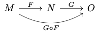
be $C^1$ maps. We want to prove the chain rule for the composition:
</p>

<p align="center">
  <img src="/blog/assets/images/composition.png" />
</p>

<h4 id="differential-of-a-map">Differential of a Map</h4>

<p>
Recall that the <b>directional derivative</b> of $F$ at $x \in M$ in the direction $v \in \R^m$ is defined to be
$$ D_vF(x) = (F\circ c)'(0), $$
where $c: I \rightarrow M$ is a $C^1$ curve such that
$$ c(0) = x\text{ and }c'(0) = v. $$
In other words, if $v \in \R^n$ is the velocity vector of a curve $c$ passing through $x \in M$, then $D_vF(x)$ is the velocity vector of the curve $F\circ c$ at $F(x)$.
</p>

<p>It is easy to check that the map
$$ v \mapsto D_vF(x) $$
is independent of the curve $c$ (as long as $c$(0)=x$ and $c'(0)=v$) and is linear. The <b>differential</b> of $F$ at $x$ is defined to be this linear map and is denoted
$$ \partial F(x): \R^m \rightarrow \R^n. $$
This is also called the <b>Jacobian</b> and often written as a matrix of partial derivatives. We avoid doing that here.
</p>

<h4 id="chain-rule">Chain Rule</h4>

<p>
Given $x \in M$, we want to find the formula for the differential of
$$ G\circ F: M \rightarrow O. $$
</p>

<p>
Given $x \in M$ and $v \in \R^m$, let $c: I \rightarrow M$ be a curve such that $c(0) = x$ and $c'(0) = v$. This in turn defines a curve
$$ F\circ c: I \rightarrow N, $$
which satisfies $(F\circ c)(0) = F(x)$ and, repeating what we said above,
\begin{align*}
(F\circ c)'(0) &amp;= \partial F(x)v.
\end{align*}
Therefore,
\begin{align*}
\partial(G\circ F)(x)v
&amp;= \left.\frac{d}{dt}\right|_{t=0}(G\circ F)(c(t))\\
&amp;= \left.\frac{d}{dt}\right|_{t=0}G((F\circ c)(t))\\
&amp;= \partial G(F(x))(F\circ c)'(0)\\
&amp;= \partial G(F(x))\partial F(x)v\\
&amp;= (\partial G(F(x))\circ\partial F(x))v
\end{align*}
This proves the chain rule
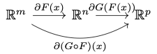
$$ \partial(G\circ F)(x) = \partial G(F(x))\circ \partial F(x), $$
</p>
<p>as depicted here:</p>

<p align="center">
  <img src="/blog/assets/images/chain_rule.png" />
</p>

<h3 id="chain-rule-for-maps-between-manifolds">Chain Rule for Maps Between Manifolds</h3>

<p>
Since everything above is done without using coordinates, the same proof works for manifolds.
</p>

<p>
 Let $M$ be an $m$-manifold, $N$ be an $n$-manifold, and $O$ be a $p$-manifold. Let
 $$F: M \rightarrow N\text{ and }G: N \rightarrow O $$
 be $C^1$ maps. We want to prove the chain rule for the composition:
</p>

<p align="center">
  <img src="/blog/assets/images/composition.png" />
</p>

<h4 id="pushforward-map">Pushforward Map</h4>

<p>
If $M$ and $N$ are manifolds, then the differential of $F$ is also called the <b>pushforward map</b>,
$$ F_*: T_xM \rightarrow T_{F(x)}N, $$
which defined as follows: For any $v \in T_xM$,
$$
F_*v = (F\circ c)'(0),
$$
where $c: I \rightarrow M$ is a $C^1$ curve such that $c(0)=x$ and $c'(0)=v$.
In other words, if $v \in T_xM$ is the velocity vector of a parameterized curve $c$ passing through $x \in M$, then $F_*v \in T_{F(x)}N$ is the velocity vector of the curve $F\circ c: I \rightarrow N$ at $F(x)$.
</p>

<h4 id="chain-rule-1">Chain Rule</h4>

<p>
Given $x \in M$, we want to find the formula for the pushforward map
$$ (G\circ F)_*: T_xM \rightarrow T_{(G\circ F)(x)}O. $$
</p>

<p>
Given $x \in M$ and $v \in T_xM$, let $c: I \rightarrow M$ be a curve such that $c(0) = x$ and $c'(0) = v$. This in turn defines a curve
$$ F\circ c: I \rightarrow N, $$
which satisfies $(F\circ c)(0) = F(x)$ and, by the definition of the pushforward map
\begin{align*}
(F\circ c)'(0) &amp;= F_*v
\end{align*}
Therefore, 
\begin{align*}
(G\circ F)_*v
&amp;= \left.\frac{d}{dt}\right|_{t=0}(G\circ F)(c(t))\\
&amp;= \left.\frac{d}{dt}\right|_{t=0}G((F\circ c)(t))\\
&amp;= G_*(F\circ c)'(0)\\
&amp;=G_*F_*v\\
&amp;= (G_*\circ F_*)v
\end{align*}
This proves the chain rule
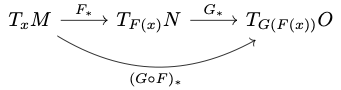
$$ (G\circ F)_* = G_*\circ F_*, $$
as depicted here:
</p>

<p align="center">
  <img src="/blog/assets/images/pushforward.png" />
</p>]]></content><author><name></name></author><category term="blog" /><category term="math" /><category term="multivariable-calculus" /><category term="maps" /><category term="chain-rule" /><category term="differential" /><summary type="html"><![CDATA[$\newcommand\R{\mathbb{R}}\newcommand\C{\mathbb{C}}\newcommand\Z{\mathbb{Z}}$]]></summary></entry><entry><title type="html">Harvard Way to Define Trace</title><link href="https://deaneyang.github.io//blog/blog/math/matrix/trace/linear-algebra/tensor-product/2024/01/11/Trace.html" rel="alternate" type="text/html" title="Harvard Way to Define Trace" /><published>2024-01-11T00:00:00+00:00</published><updated>2024-01-11T00:00:00+00:00</updated><id>https://deaneyang.github.io//blog/blog/math/matrix/trace/linear-algebra/tensor-product/2024/01/11/Trace</id><content type="html" xml:base="https://deaneyang.github.io//blog/blog/math/matrix/trace/linear-algebra/tensor-product/2024/01/11/Trace.html"><![CDATA[<p>$\newcommand\F{\mathbb{F}}\newcommand\R{\mathbb{R}}\newcommand\C{\mathbb{C}}\newcommand\Z{\mathbb{Z}}\newcommand\tr{\operatorname{trace}}\newcommand\End{\operatorname{End}}$</p>
<p>
The trace of a sqaure matrix $A$ is defined to be the sum of the elements along the diagonal. A basic fact is that for any invertible matrix $M$,
\begin{equation}\tag{*} \tr(M^{-1}AM) = \tr(A). \end{equation}
</p>

<p>
Let $V$ be an $n$-dimensional vector space over a field $\F$.
The trace of a linear transformation $L: V \rightarrow V$ is usually defined as follows:
Let $(v_1, \dots, v_n)$ be a basis of $V$. There exists a matrix $A$ such that
$$ L(e_i) = A_i^je_j. $$
Then the trace of $L$ is defined to be
$$ \tr(L) = \tr(A). $$
Fact (*) implies that this the right side remains the same, no matter which basis of $V$ is used.
</p>

<p>
A natural question is whether there is a way to define the trace of a linear transformation directly without using a basis or matrix. This would prove (*). One way is to use the universal property of the tensor product of two vector spaces.
</p>

<p>
<b>Universal property of tensor product:</b> Let $V$ and $W$ be vector spaces over a field $\F$. The tensor product $V\otimes W$ is a vector space with a bilinear map
\begin{align*}
B: V\times W &amp;\rightarrow V\otimes W\\
(v,w) &amp;\mapsto v\otimes w
\end{align*}
such that the following universal property holds: For any vector space $Z$ and bilinear map
$$ b: V\times W \rightarrow Z, $$
there exists a unique linear map
$$ \bar{b}: V\otimes W \rightarrow Z $$
such that
$$
b = \bar{b}\circ B.
$$
</p>

<p>
<b>Space of linear transformations is tensor product:</b>
Let $\End(V)$ denote the space of linear transformations from $V$ to itself. The set of all rank $1$ linear transformations is the image of the following bilinear map
\begin{align*}
\phi: V \times V^* &amp;\rightarrow \End(V),
\end{align*}
where for any $(v,\ell) \in V\times V^*$, the map $\phi(v,\ell): V \rightarrow V$ is the rank $1$ map such that for aany $w \in V$ to be
$$ \phi(v, \ell)(w) = (\ell(w))v. $$
By the universal property above, this extends uniquely to a linear map
$$ \bar\phi: V\otimes V^* \rightarrow \End(V). $$
It is straightforward to verify that $\bar\phi$ is an isomorphism.
</p>

<p>
<b>Trace of linear transformation:</b>
The trace of any rank 1 linear transformation is given by the following natural bilinear function
\begin{align*}
e: V \times V^* &amp;\rightarrow \F\\
(v,\ell) &amp;\mapsto \ell(v)
\end{align*}
By the universal property above, this extends uniquely to a linear map
$$
\bar{e}: V\otimes V^* \rightarrow \F.
$$
The trace of a linear transformation $L \in \End(V)$ can now be defined to be
$$
\tr(L) = \bar{e}\circ\bar{\phi}^{-1}(L).
$$
</p>

<p>
<em>Acknowledgement:</em> This post was inspired by <a href="https://web.math.princeton.edu/generals/alpoge_levent">Levent Alpoge's Princeton PhD generals exam</a>. Just look for "Harvard way".
</p>]]></content><author><name></name></author><category term="blog" /><category term="math" /><category term="matrix" /><category term="trace" /><category term="linear-algebra" /><category term="tensor-product" /><summary type="html"><![CDATA[$\newcommand\F{\mathbb{F}}\newcommand\R{\mathbb{R}}\newcommand\C{\mathbb{C}}\newcommand\Z{\mathbb{Z}}\newcommand\tr{\operatorname{trace}}\newcommand\End{\operatorname{End}}$ The trace of a sqaure matrix $A$ is defined to be the sum of the elements along the diagonal. A basic fact is that for any invertible matrix $M$, \begin{equation}\tag{*} \tr(M^{-1}AM) = \tr(A). \end{equation}]]></summary></entry><entry><title type="html">Singular Value Decomposition</title><link href="https://deaneyang.github.io//blog/blog/math/matrix/matrices/linear-algebra/singular-values/2023/01/05/Singular-Value-Decomposition.html" rel="alternate" type="text/html" title="Singular Value Decomposition" /><published>2023-01-05T00:00:00+00:00</published><updated>2023-01-05T00:00:00+00:00</updated><id>https://deaneyang.github.io//blog/blog/math/matrix/matrices/linear-algebra/singular-values/2023/01/05/Singular-Value-Decomposition</id><content type="html" xml:base="https://deaneyang.github.io//blog/blog/math/matrix/matrices/linear-algebra/singular-values/2023/01/05/Singular-Value-Decomposition.html"><![CDATA[<p>$\newcommand\R{\mathbb{R}}\newcommand\C{\mathbb{C}}\newcommand\Z{\mathbb{Z}}$</p>

<p>The singular value decomposition is usually defined for a matrix. Here, we will show directly that any linear map between inner product spaces has a singular value decomposition. The singular value decomposition of a matrix follows by letting the inner product spaces be $\R^n$ or $\C^n$ with the standard inner product. Only real inner product spaces will be considered here, but the complex case is almost exactly the same.</p>

<p>Let $M$ be an $m$-dimensional real inner product space, $N$ be an $n$-dimensional real inner product space, and $L: M \rightarrow N$ be a linear map.</p>

<p>
We start with a geometric description of a singular value decomposition of $L$. A singular value decomposition of $L$ consists of an orthonormal basis $(v_1, \dots, v_m)$ of $M$ and an orthonormal basis $(u_1, \dots, u_n)$ of $N$, and positive real scalars $\lambda_1, \dots, \lambda_r$, where $r$ is the rank of $L$, such that the following hold:
<ul>
<li>$(v_{r+1}, \dots, v_m)$ is a basis of $\ker(L)$</li>
<li>$(u_{r+1}, \dots, u_n)$ is a basis of $(\operatorname{image}(L))^\perp$</li>
<li>$L(v_j) = \lambda_ju_j$ for each $1 \le j \le r$</li>
</ul>
The distinct values of $\lambda_1, \dots, \lambda_r$ are called the <b>singular values</b> of the map $L$.
</p>

<p>
Equivalently, a <b>singular value decomposition</b> of $L$ is
$$
L = U\Sigma V^*,
$$
where $V: \R^m \rightarrow M$ and $U: \R^n\rightarrow N$ are isometries and $\Sigma$ is a diagonal $n$-by-$m$ matrix such that
\begin{align*}
  \Sigma_j^j &amp;= \lambda_j \text{ if }1 \le j \le r\\
  \Sigma_j^a &amp;= 0\text{ otherwise}.
\end{align*}
</p>

<p>
The equivalence follows by observing that if $1 \le j \le r$, then
\begin{align*}
  U\Sigma V^*(v_j)
  &amp;=   U\Sigma e_j\\
  &amp;= \lambda_j Ue_j\\
  &amp;= \lambda_j u_j
\end{align*}
and if $r+1 \le j \le m$, then
\begin{align*}
  U\Sigma V^*(v_j)
  &amp;= U\Sigma e_j\\
  &amp;= 0.
\end{align*}
</p>

<p>A singular value decomposition of any linear map $L: M \rightarrow N$ can be constructed as follows:</p>

<p>The linear map $L^*L$ is nonnegative-definite and self-adjoint and therefore has  nonnegative real eigenvalues $\lambda_1^2, \dots, \lambda_m^2$. We can assume that $\lambda_1, \dots, \lambda_r &gt; 0$ and $\lambda_{r+1}, \dots, \lambda_m = 0$. Let $s_1, \dots, s_k$ be the distinct values of $\lambda_1, \dots, \lambda_r$.</p>

<p>
The eigenspaces of $L^*L$ are mutually orthogonal. Denote the dimensions of the eigenspaces for $s_1^2, \dots, s_k^2$ by $d_1, \dots, d_k$, respectively. Observe that
$$
  r = d_1 + \cdots + d_k
$$
is the rank of $L$. 
Given an ordering of the singular values, we can assume that the ordering of $\lambda_1, \dots, \lambda_m$ is given by
\begin{align*}
\lambda_{d_1+\cdots+d_{j-1}+1}=\cdots=\lambda_{d_1+\cdots+d_{j-1}+d_j}&amp;= s_j\text{ for each }1 \le j \le r\\
\lambda_{r+1} = \cdots \lambda_m &amp;= 0.
\end{align*}
</p>

<p>
Let $(v_1, \dots, v_m)$ be an orthonormal basis of $M$ of eigenvectors of $L^*L$, where each $v_j$ is an eigenvector for the eigenvalue $\lambda_j$.  Let $V: \R^m \rightarrow M$ be the linear map such that
$$
V(e_j) = v_j,\ 1 \le j \le m,
$$
where $(e_1, \dots, e_m)$ is the standard basis of $\R^m$.
</p>

<p>
For each $1 \le j \le r$, let
\[
  \bar{u}_j = L(v_j) \in N.
\]
For each $1 \le i, j \le r$,
\begin{align*}
  \langle \bar{u}_i,\bar{u}_j\rangle &amp;= \langle L(v_i), L(v_j)\rangle\\
                                     &amp;= \langle v_i, L^*L(v_j)\rangle\\
                                     &amp;= \lambda_j^2 \langle v_i,v_j\rangle\\
                                     &amp;= \lambda_j^2\delta_{ij}.
\end{align*}
Since $\lambda_1, \dots, \lambda_r &gt; 0$, it follows that
$$
u_1 = \frac{\bar{u}_1}{\lambda_1}, \dots, u_r = \frac{\bar{u}}{\lambda_r}
$$
is an orthonormal basis of $\operatorname{image}(L) \subset N$. This can be extended to an orthonormal basis $(u_1, \dots, u_n)$ of $N$. By their construction, the bases $(v_1, \dots, v_m)$ and $(u_1, \dots, u_n)$ satisfy the geometric definition of a singular value decomposition of $L$.

<p>
If we now define $V: \R^m \rightarrow M$ and $U: \R^n \rightarrow N$ such that
\begin{align*}
V(e_j) &amp;= v_j,\ 1 \le j \le m\\
U(e_a) &amp;= u_a,\ 1 \le a \le n,
\end{align*}
then they satisfy the second definition of a singular value decomposition.
</p>

A natural question is to what extent are $U$ and $V^*$ unique. It is clear from the above construction that if we fix an ordering of the singular values $s_1, \dots, s_k$ and the corresponding ordering of $\lambda_1, \dots, \lambda_r$, as specified above, then $V$ is unique up to rotations in each eigenspace of $L^tL$ and, given $V$, $U$ is unique up to rotations of $(\operatorname{image}(L))^\perp$.


</p>]]></content><author><name></name></author><category term="blog" /><category term="math" /><category term="matrix" /><category term="matrices" /><category term="linear-algebra" /><category term="singular-values" /><summary type="html"><![CDATA[$\newcommand\R{\mathbb{R}}\newcommand\C{\mathbb{C}}\newcommand\Z{\mathbb{Z}}$]]></summary></entry><entry><title type="html">Visualization of Moore-Penrose Pseudoinverse</title><link href="https://deaneyang.github.io//blog/blog/math/linear-algebra/matrix/moore-penrose/2022/12/16/MoorePenrose.html" rel="alternate" type="text/html" title="Visualization of Moore-Penrose Pseudoinverse" /><published>2022-12-16T00:00:00+00:00</published><updated>2022-12-16T00:00:00+00:00</updated><id>https://deaneyang.github.io//blog/blog/math/linear-algebra/matrix/moore-penrose/2022/12/16/MoorePenrose</id><content type="html" xml:base="https://deaneyang.github.io//blog/blog/math/linear-algebra/matrix/moore-penrose/2022/12/16/MoorePenrose.html"><![CDATA[<p>$\newcommand\R{\mathbb{R}}\newcommand\C{\mathbb{C}}\newcommand\Z{\mathbb{Z}}$</p>

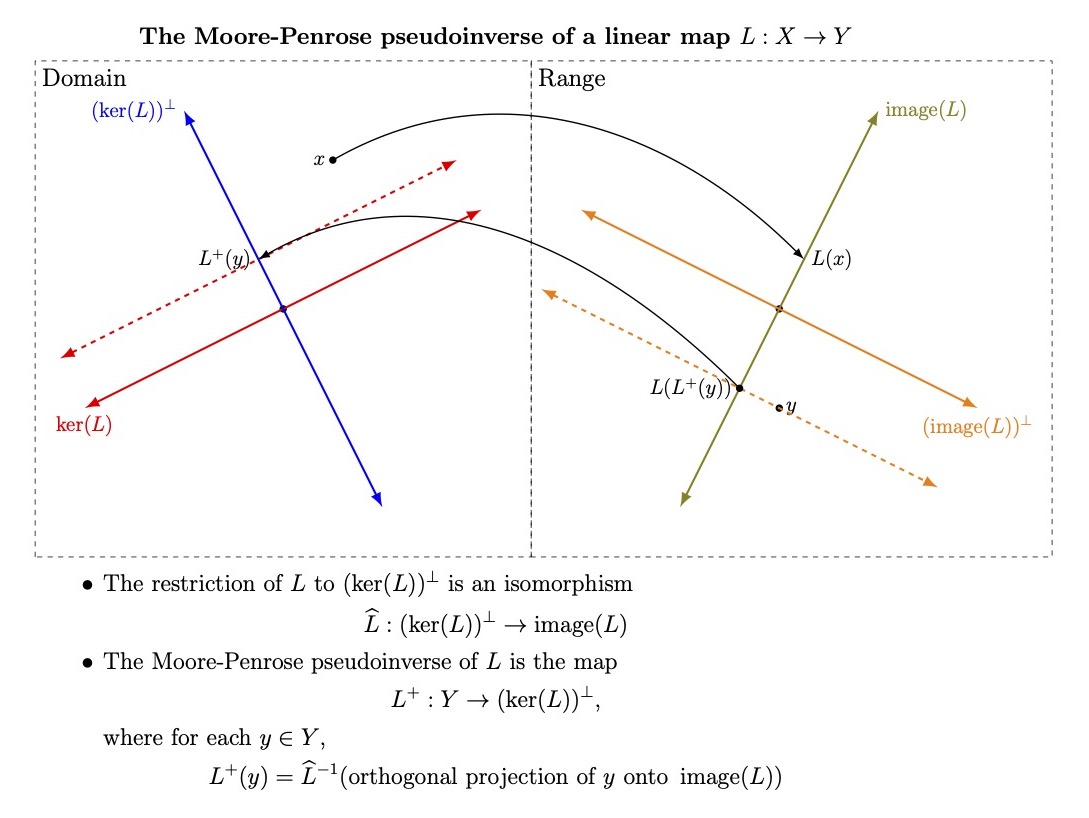
<p align="center">
  <img src="/blog/assets/images/moore-penrose.jpg" />
</p>]]></content><author><name></name></author><category term="blog" /><category term="math" /><category term="linear-algebra" /><category term="matrix" /><category term="moore-penrose" /><summary type="html"><![CDATA[$\newcommand\R{\mathbb{R}}\newcommand\C{\mathbb{C}}\newcommand\Z{\mathbb{Z}}$]]></summary></entry><entry><title type="html">Orientation of a manifold</title><link href="https://deaneyang.github.io//blog/blog/math/differential-geometry/manifolds/2022/06/04/OrientationManifold.html" rel="alternate" type="text/html" title="Orientation of a manifold" /><published>2022-06-04T00:00:00+00:00</published><updated>2022-06-04T00:00:00+00:00</updated><id>https://deaneyang.github.io//blog/blog/math/differential-geometry/manifolds/2022/06/04/OrientationManifold</id><content type="html" xml:base="https://deaneyang.github.io//blog/blog/math/differential-geometry/manifolds/2022/06/04/OrientationManifold.html"><![CDATA[<p>
$\newcommand\R{\mathbb{R}}$
$\newcommand\extV{\Lambda^nV^*}$
$\newcommand\extVo{\Lambda^nV^*\backslash\{0\}}$
$\newcommand\extT{\Lambda^nT^*M}$
</p>

<p>It always starts with linear algebra. I like to say that differential geometry is the study of parameterized families of vector spaces.</p>

<h3 id="orientation-of-a-vector-space">Orientation of a vector space</h3>

<p>The first observation is that a $1$-dimensional vector space with the origin removed has two connected components. There is no natural way of labeling one as positive and the other as negative. The second observation is that if $V$ is an $n$-dimensional vector space, then the vector space $\extV$ of exterior $n$-tensors is $1$-dimensional.</p>

<p>An orientation on $V$ is defined by choosing one of the connected components of $\extVo$. Let’s call that component $\extV_+$. Given any nonzero $\Theta \in \extV$, we say that $\Theta$ has positive orientation if $\Theta \in \extV_+$ and negative orientation otherwise.</p>

<p>Conversely, any nonzero $\Theta \in \extV$ uniquely determines an orientation on $V$ by letting $\extV_+$ be the connected component of $\extVo$ that contains $\Theta$.</p>

<p>Also, note that $\Theta_1, \Theta_2 \in \extVo$ have the same orientation if and only if $\Theta_2 = c \Theta_1$ for some $c &gt; 0$.</p>

<h3 id="orientation-of-a-manifold">Orientation of a manifold</h3>

<p>Now let $M$ be a smooth manifold. We say that $M$ is orientable if there exists a continuous nowhere zero exterior $n$-form $\Theta$ on $M$. If such an form exists, then it uniquely determines an orientation on each $T_pM$, $p \in M$.</p>

<p>Any nowhere zero $n$-form on a connected oriented manifold is either positively or negatively oriented. If the manifold is not connected, then the form has a sign on each connected component but the signs do not have to be the same.</p>

<h3 id="volume-form">Volume form</h3>

<p>A volume form on $M$ is defined to be a continuous nowhere zero $n$-form. If $M$ is connected and oriented, then a volume form is either positively or negatively oriented.</p>

<h3 id="integral-of-a-volume-form">Integral of a volume form</h3>

<p>The definition of the integral of a volume form on an $n$-dimensional manifold has an ambiguity in its sign. If the manifold is oriented, then the ambiguity is resolved as follows:</p>

<p>If a volume form is positively oriented, then the sign of its integral is chosen to be positive. If it has negative orientation, then the sign is chosen to be negative.</p>

<p>More generally, if $\Theta$ is a volume form and $f$ is a continuous nonnegative function on $M$, then the sign of
\(\int_M f\Theta\)
is chosen to be nonnegative.</p>

<h3 id="integral-of-an-n-form">Integral of an $n$-form</h3>

<p>
Let $\Theta$ be a positively oriented volume form on an oriented manifold $M$. If $\Omega$ is a continuous $n$-form, there is a continuous function $f$ on $M$ such that $\Omega = f\Theta$. If we let $f_+$ and $f_-$ denote the positive and negative parts of $f$, then we define the integral of $\Omega$ to be
$$
\int_M \Omega = \int_M f_+\Theta - \int_M f_-\Theta.
$$
</p>

<p>It is now clear that if $M$ is oriented but not connected, then for any $c \in \R$ there exists a volume form $\Theta$ such that
\(\int_M \Theta = c.\)</p>]]></content><author><name></name></author><category term="blog" /><category term="math" /><category term="differential-geometry" /><category term="manifolds" /><summary type="html"><![CDATA[$\newcommand\R{\mathbb{R}}$ $\newcommand\extV{\Lambda^nV^*}$ $\newcommand\extVo{\Lambda^nV^*\backslash\{0\}}$ $\newcommand\extT{\Lambda^nT^*M}$]]></summary></entry><entry><title type="html">The definition of a manifold</title><link href="https://deaneyang.github.io//blog/blog/math/differential-geometry/manifolds/2022/03/22/DefinitionManifold.html" rel="alternate" type="text/html" title="The definition of a manifold" /><published>2022-03-22T00:00:00+00:00</published><updated>2022-03-22T00:00:00+00:00</updated><id>https://deaneyang.github.io//blog/blog/math/differential-geometry/manifolds/2022/03/22/DefinitionManifold</id><content type="html" xml:base="https://deaneyang.github.io//blog/blog/math/differential-geometry/manifolds/2022/03/22/DefinitionManifold.html"><![CDATA[<p>$\newcommand{\R}{\mathbb{R}}$
I’ve always disliked the standard ways to define a manifold in differential geometry. First, the definition always starts with a topological space $M$. I don’t understand why you need make this assumption. I prefer to show that the topology of $M$ is a natural consequence of the definition. Second, the definition always uses two technical terms, paracompact and Hausdorff. I prefer to describe the properties concretely in terms of coordinate maps.</p>

<p>Below is how I prefer to define a manifold. It turns out that Peter Olver, in his book <em>Applications of Lie Groups to Differential Equations</em> (published in 1986) defines a manifold in exactly the same way (see Definition 1.1).</p>

<p>Start with a set $M$, just a set. Define a coordinate map to be a bijection $\phi: O \rightarrow \mathbb{R}^n$, where $O$ is a subset of $M$ and $\phi(O) \subset \mathbb{R}^n$ is open. Define an atlas to be a countable collection of coordinate maps, where the domains of the maps cover $M$. No assumptions about topology or smoothness yet.</p>

<p>A topological atlas is one where for any two coordinate maps $\phi_1: O_1 \rightarrow \mathbb{R}^n$ and $\phi_2: O_2\rightarrow \mathbb{R}^n$ such that $O_1\cap O_2 \ne \emptyset$, the change of coordinate map</p>

\[\phi_2\circ\phi_1^{-1}: \phi_1(O_1\cap O_2) \rightarrow \phi_2(O_1\cap O_2)\]

<p>is a homeomorphism. A topological manifold is a set $M$ with a topological atlas.</p>

<p>Observe that this defines a topology on $M$, where any coordinate map $\phi: O \rightarrow \phi(O) \subset \R^n$ is a homeomorphism. The assumption on the change of coordinate maps is exactly what is needed for this definition to be logically consistent.</p>

<p>Usually (but not always), there is one more assumption made, which I like to state as follows:</p>

<p><i>You can separate points using coordinate charts.</i></p>

<p>More precisely, given two different points $p_1, p_2 \in M$, there exist coordinate maps $\phi_1: O_1\rightarrow \R^n$, $\phi_2: O_2\rightarrow \R^n$ and open subsets $U_1 \subset O_1$, $U_2\subset O_2$ such that</p>
<ul>
  <li>$p_1 \in U_1$ and $p_2 \in U_2$</li>
  <li>$U_1\cap U_2 = \emptyset$</li>
</ul>

<p>The fact that the atlas has countably many coordinate maps is equivalent to $M$ being paracompact. The fact that points can be separated by coordinate charts is equivalent to $M$ being Hausdorff.</p>

<p>The definition of a smooth manifold is exactly the same, except that the change of coordinate maps are also assumed to be smooth, i.e., diffeomorphisms.</p>]]></content><author><name></name></author><category term="blog" /><category term="math" /><category term="differential-geometry" /><category term="manifolds" /><summary type="html"><![CDATA[$\newcommand{\R}{\mathbb{R}}$ I’ve always disliked the standard ways to define a manifold in differential geometry. First, the definition always starts with a topological space $M$. I don’t understand why you need make this assumption. I prefer to show that the topology of $M$ is a natural consequence of the definition. Second, the definition always uses two technical terms, paracompact and Hausdorff. I prefer to describe the properties concretely in terms of coordinate maps.]]></summary></entry></feed>